Good Things Come to Those Who Can’t Wait, Part 1
This post was coauthored with Allen Sirolly and is the first post in our two-part series on arrival rate bias correction in A/B Testing. We are very grateful to our Wealthfront Data Science colleague, Hsiu-Chi Lin, for his invaluable input. Part 2 may be found here.
Like many technology companies, Wealthfront uses in-product testing and experimentation to learn and make decisions. In particular, we leverage in-product A/B testing of our existing client base to understand how product decisions cause changes in behavior. However, there are characteristics of our product and business that complicate conducting these experiments and making valid inferences from their results. For example, measuring effects at the client level, rather than the session level, requires care. As does the measurement of effects that can that can take days or weeks to materialize, as opposed to manifesting contemporaneously with treatments. Lastly, a challenge specific to in-product testing of existing clients stems from compliance bias driven by heterogeneity in product usage rates. This phenomenon, which we refer to as “Arrival Rate Bias”, is the topic of our next two posts. In part 1, we cover the following sections:
Define the problem
Operationalize arrival rates
Show how this bias manifests in a real experiment
Introduce potential solutions
In Part 2, we will dig deeper into details of our implemented solution and discuss its implications for power calculations.
The Problem
As a form of Randomized Control Trial (RCT) A/B testing requires that observations be sampled randomly. While this fairly obvious requirement is easy enough to explain, it can be harder to implement in practice than anticipated. For example, it can be difficult to simply ensure that observations are split randomly between control and treatment groups. This can be particularly challenging when A/B testing on mobile devices, where users in the treatment group (but not the control) need to upgrade their app to be exposed to a variant. However, less attention appears to have been paid to bias introduced during sample selection prior to random assignment.
Bucketing
When running in-product A/B tests we first randomly “assign” all existing clients to either the control or treatment experience. In principle, this random assignment should give us an unbiased estimate of the average treatment effect (ATE). However, it isn’t until a client actually logs in on either web or mobile that they are “bucketed” into a given experiment. We make inferences on this sample of bucketed clients to avoid diluting measured effect sizes due to non-exposure. However, this mechanism introduces bias into our aggregate experiment samples as clients who log in more frequently are more likely to be bucketed. Therefore, these clients are overrepresented in our samples and are bucketed earlier into experiments, on average. Furthermore, if a client’s propensity to “arrive” at Wealthfront is related to their propensity to respond to our experiments then there could be selection bias in our measured ATE. For example, if younger clients (in terms of biological age) log in more often than older clients, and if this younger cohort is more likely to positively respond to changes we make to our UI, then we might expect to see bias introduced by the age confounder.
We have evidence that this kind of thing may be happening. Our Financial Planning team recently ran an experiment to more clearly merchandise our home planning feature. The aim of this test was to see if we could increase the proportion of our clients who created home planning goals while avoiding any negative impact on other metrics such as retention and engagement. Using our in-house A/B testing platform, which provides real-time monitoring of bucketing and treatment effects, we observed an ATE time series like this:
This issue may exist for any company measuring effect sizes at the user-level, but arrival rate bias is particularly acute for Wealthfront for three reasons. Most importantly, our clients exhibit significant heterogeneity in their arrival rates: many clients log in once a month or once a quarter to check up, while others log in daily and pay closer attention to their portfolios. In addition, our clients log in relatively infrequently as compared to other digital products (perhaps acting on our advice to “set it and forget it”.) Lastly, the issues caused by the nature of our clients’ arrival rate distribution are exacerbated by the fact that we are often measuring treatment effects that materialize over periods of weeks or longer. For example, rolling over a 401(k) account isn’t something a client can do completely in the app, and once the process starts it can take weeks to complete. And our Portfolio Line of Credit feature is typically used by clients to cover large but infrequent liquidity needs, which means that any effect we have on their usage won’t be measured quickly.
Arrival Rate
In order to study the relationship between the unobserved arrival propensity and its effect on our experimental inferences, we define an ex-ante observed measure that is predictive of a client’s ex-post time of arrival (X). These “arrival rates” can be estimated from a client’s recent session history prior to the start of a given experiment. We denote the arrival rate measure as lambda (λ) with reference to the rate parameter of a Poisson process. An unbiased estimate of this parameter is the inverse of the time since a user’s second-to-last session before the start of the experiment (T) (where S_k is the time of the kth-to-last session):
This definition has the advantage of being continuous. And the number of sessions considered is small enough to effectively proxy for a client’s instantaneous arrival rate, which we know to be important because we have evidence that arrival rates are time-varying. Importantly, these heuristic calculations of λ_i only make use of a user’s session history prior to the start of an experiment rather than prior to the time of bucketing. This is intentional, as λ_i and the time until bucketing should be independent when making claims about the relationship between the two.
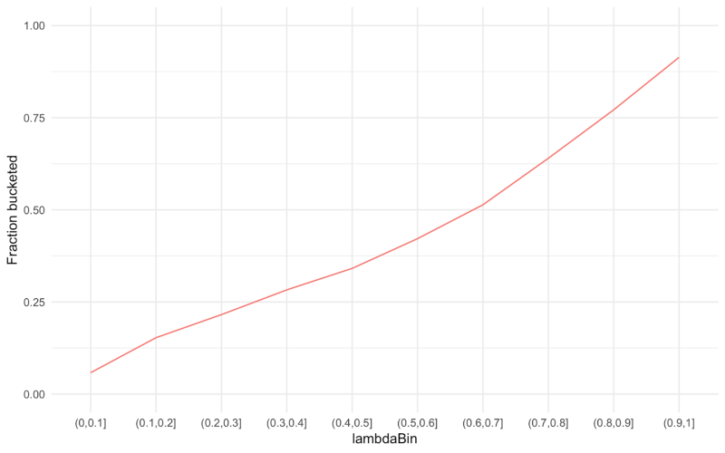
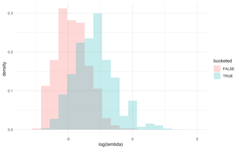
The above plot demonstrates that λ, an ex-ante estimate, can accurately capture ex-post arrival propensity by demonstrating that λ is positively and monotonically related to the fraction of clients that we bucketed into our home planning experiment. Finally, it is clear when we compare the arrival rate distributions of clients who were bucketed into the experiment with those that were not that there is a meaningful selection effect.
Quantifying Arrival Rate Bias
The second necessary condition for arrival rate bias is a differential effect size as a function of λ. If frequent arrivers and infrequent arrivers are just as likely to modify their behavior in response to our experiments, then we have nothing to worry about. But if they react differently then the ATE will likely be biased. We can estimate treatment effect heterogeneity in our home planning experiment using logistic regression:
Where Z equals 1 if a client is in the treatment group and 0 otherwise. We choose this form as our experiment measured the proportion of clients who created a home planning goal. If we plot the response functions for the treatment and control groups, we see evidence of heterogeneity:
One explanation for this is that λ is correlated with observables — tenure, age, net worth, income — which are more directly related to client behavior. In fact, we know this to be the case. In addition, high-λ clients in the treatment group have more opportunities to take action after being bucketed as they are exposed to our treatments more frequently.
To estimate the severity of arrival rate bias in this example, we can compute the ATE using the predicted values of the model with values sampled from the population distribution of λ. Standard errors for the predicted counterfactual means are bootstrapped. We observe that the ATE under the sample of bucketed clients matches the observed average effect size, giving us confidence in the accuracy of our model. The lower predicted effect size for the population of clients is consistent with both the increasing effect size in the response plot above and the decreasing ATE in the first plot from this post.
A Simple Hierarchical Model
We can further explore how the severity of arrival rate bias changes with the fraction of samples collected. At this point, it is instructive to write down a simple hierarchical model. Suppose each client’s arrival rate is drawn from some distribution F_λ, and their first arrival time X_i from an exponential distribution (the Poisson assumption):
Visual inspection shows that LogNormal(μ, σ²) is a reasonable parametrization for F_λ. The chart below shows the maximum likelihood fit to the empirical population distribution of λ for our home planning experiment:
Then we define K as the number of clients randomly assigned to our experiment, N as the cumulative number who arrive and are bucketed, and R := N / K as the proportion of assigned clients bucketed at a given time. Using the fitted distribution, we can easily compute the arrival-biased distribution conditional on R. Integrating the estimated effect function τ(λ) over the biased distribution H_λ(λ; R), we can estimate the relative bias B(R) for any value of R and not just the R* that was realized (the fraction of clients who were actually bucketed into the experiment). Below we plot the relative bias
as a function of R for our home planning experiment. Note that as R approaches 1 bias approaches 0. We see that a naive interpretation of the estimated lifts from these experiments would yield significantly biased inferences.
Potential Solutions
We consider three possible solutions to the issue of arrival rate bias. First, the regression approach used to quantify the bias above can be adapted to correct for it, by controlling for confounding variables. However, this would only control for observables, while the methods we investigate below allow us to also control for unobservables (because we know the bucketing mechanism). Second, we randomly preselect clients to be included in an experiment and wait for some proportion of these clients to arrive at the site. Lastly, we reweight the responses of clients who arrive and are bucketed into our experiment to approximate the distribution of our overall client base. For “doubly robust” estimators that combine regression and propensity weighting, see this article.
Preselection
In a world in which time is not a constraint, we would prefer to preselect K existing clients and wait for all of them to arrive at the site. This would give us an unbiased sample with respect to our existing client base at the time an experiment is launched. But, as previously discussed, it would take months for all of these K clients to arrive and we need to make causal inferences on a shorter timescale.
One workaround is to trade off bias for time by measuring the effect size on the first N of K clients that arrive. Recognizing that the bias in our estimate declines as R increases allows us to make informed decisions about how much bias we are willing to accept and whether this will allow us to collect the samples we need in the time allotted to an experiment. For example, we might randomly sample K = 20,000 clients and wait for the first N = 15,000 of them to be bucketed (R = .75). This R implies some amount of expected bias, which can be reduced simply by increasing R. This approach has the benefit that the time to wait for the Nth client to arrive only depends on R, and not on N or K individually.
The relative bias plot for our home planning experiment presented in the previous section shows that the number of samples we actually collected implied a relative bias of roughly 20 percent — more than we are comfortable tolerating. We could have waited for more samples to arrive, but the closer R is to 1, the longer it would have taken to collect our sample. Given that we have clients who log in monthly, quarterly and even less frequently, this is not feasible. In addition, preselection is not amenable to real-time monitoring as it only converges to the right answer as R approaches 1, while we want an unbiased estimate of the ATE at every time step. Fortunately, this is a characteristic of our next approach to solving the problem.
Inverse Propensity Weighting
Weighted sampling is another possible solution to the problem of arrival rate bias. Various approaches to sample reweighting can be found in the causal inference literature. These reweighting methods allow for robust and flexible causal modeling in the case of selection on observables but, as previously mentioned, they do not eliminate bias due to unobserved confounding. However, our knowledge of the bucketing mechanism allows us to directly control for these unobserved factors.
The specific approach we implemented is known as Inverse Propensity Weighting (IPW). We underweight clients with high arrival rates (those disproportionately likely to be bucketed) and overweight clients with low arrival rates. By selecting appropriate weights, we can sample as if from the unbiased distribution. To illustrate this point, let’s revisit the hierarchical model described earlier. Suppose that the population distribution of λ has a density f_λ(λ) and that the marginal distribution of arrival times X has distribution G_X(x). Then the arrival-biased distribution of λ has some density h_(λ|X≤Z)(λ), where Z := G_X^-1(R) (using an asymptotic argument for X_(N), the time of the Nth bucketing/arrival). We would like a weight function which transforms h into f:
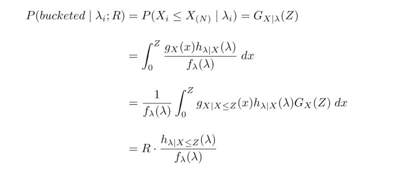
This is precisely the likelihood ratio f_λ(λ) / h_(λ|X≤Z)(λ; R). A more useful expression is:
Where the denominator denotes the probability that a client with arrival rate λ_i will be bucketed by the time that R = N / K samples have been collected. A little bit of math shows that this expression is equivalent to the likelihood ratio:
Intuitively, the weight is smaller for clients who are likely to be bucketed (because they have high arrival rates there are disproportionately more of them in our sample), and larger for those who are less likely to be bucketed. The fact that the propensity is a function of R means that the weights give us an unbiased estimate of the ATE for any number of samples collected — a crucial property that we need for our real-time monitoring setup.
Next Steps
While it solves our original problem, IPW introduces a tradeoff. Namely, while we can recover an unbiased estimate of the ATE, the variance of the estimator is amplified by the weights. This means we need a larger sample size for a given experiment to achieve some set target of statistical power. A critical question to answer is “How much larger?” In the second part of this post, we will provide a solution and document the effect of the IPW correction on simulated and actual experiments.


